library(mrgsolve)
library (dplyr)
library (nloptr)
library (ggplot2)

Fitting a PK model in R using mrgsolve

In this blog post, we will start by briefly reviewing the components needed to opimize parameters in the context of pharmacokinetic/pharmacodynamic models, then continue with an example.

Introduction

To optimize the parameters of our model, we’ll need an objective function (which we’ll aim to minimize), a parameter search algorithm, and an odinary differential equation (ODE) solver.

Model and data
- In the context of PK/PD modeling, the model is typically defined by a series of differential equations. Thus a differential equation solver is needed. Some common solvers include LSODA, Runge-Kutta, LSODI, and Euler’s method.
Objective Function
- Maximum Likelihood
- Least Squares
- Weighted Least Squares
- MAP Bayes
Parameter Search Algorithm
- Nelder-Mead
- Gradient Descent
- Grid-search
- Many others (simulated annealing, genetic algortihm, etc.)

PK Model

We’ll use a simple 1 compartment PK model with proportional residual error.

code <- '
$PROB 1 cmt PK Model

$PARAM
CL=1
VC = 20
KA=0.6
sigma1 = 0.1

$CMT X1 X2 


$ODE
dxdt_X1 = -KA*X1;
dxdt_X2 = KA*X1 - CL/VC*X2;


$TABLE
double Y1 = X2/VC;
double varY1 = (Y1*sigma1)*(Y1*sigma1);

$CAPTURE Y1 varY1 
'

mod<-mcode(code=code)

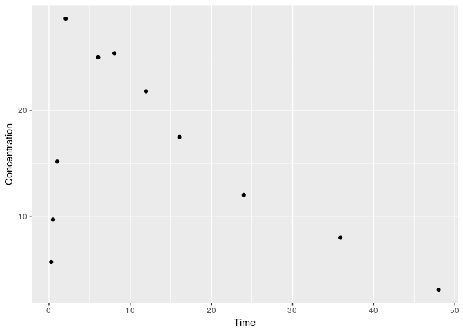
Let’s read in our observed data. The first column is time, and each subsequent column corresponds to an output (Y1, Y2, …) defined in our model. In this case, just one output, Y1:

data <-read.csv("data.csv",header = F)
head(data)

.       V1      V2
. 1 0.2864  5.7460
. 2 0.5155  9.7379
. 3 1.0309 15.1815
. 4 2.0619 28.6089
. 5 6.0710 24.9798
. 6 8.0756 25.3427

print(ggplot(data,aes(x=V1,y=V2))+
        geom_point()+
        labs(x="Time", y= "Concentration"))

and the dosing data:

rawdose<- read.csv("dosing-data.csv")
dose <- mutate(rawdose,ID=1,evid=1)
head(dose)

.   time  amt cmt ID evid
. 1    0 1000   1  1    1

We’ll define a function to output predictions at observed time points, given a set of parameters, dosing profile, and model.

pred<- function(params,observed,dosing,mod,param_names=names(params)){
  time <- as.vector(observed[,1])
  params_list<-as.list(params)
  names(params_list)<- param_names
  output.names <- paste0("Y",1:dim(observed)[1])
  var.output.names <- paste0("varY",1:dim(observed)[1])
  
  
  out<-mod %>%
    data_set(dose)%>%
    param(params_list)%>%
    obsonly()%>%
    mrgsim(end = -1, add = time)
  outindex <- which (names(out@data)%in%output.names) #search output of mrgsolve model for Y1, Y2, etc.
  varoutindex <- which (names(out@data)%in%var.output.names) #search output of mrgsolve model for varY1, varY2, etc.
  list(as.vector(unlist(out@data[outindex])),as.vector(unlist(out@data[varoutindex])))
}                                           

Objective Function - Maximum Likelihood

We will be using the maximum likelihood objective function. Assuming the residual errors for all observations are normally distributed and independent, the -2 log likehood becomes:

$-2LL = \frac{1}{2}*n_{obs}*ln(2\pi)+\displaystyle\sum_{i=1}^{n}\Big(\dfrac{(y_{obs,i}-y_{pred,i})^2}{\sigma_{pred,i}}+ln(\sigma_{pred,i})\Big)$

Let’s define it in an R function:

MLObjFun <- function(params,observed,dosing,mod,param_names){
  a<-pred(params,observed,dosing,mod,param_names)
  obs<-as.vector(unlist(observed[-1]))

  1/2*sum(((a[[1]]-obs)*(a[[1]]-obs))/a[[2]]+log(a[[2]]))+1/2*length(obs)*log(2*pi)
}

Optimizer - Nelder-Mead

To optimize the parameters, we’ll use the Nelder-Mead algorithm from the nloptr package.

theta <- c(CL=1,VC=10,KA=0.6)
sigma <- c(sigma1 = 0.1)
params = c(theta,sigma)

fit <-neldermead(x0=params,fn=MLObjFun,observed=data,dosing=dose,mod=mod,param_names =names(params))

print(fit)

. $par
. [1]  1.3654867 28.0853974  0.6280271  0.1009130
. 
. $value
. [1] 18.64377
. 
. $iter
. [1] 278
. 
. $convergence
. [1] 4
. 
. $message
. [1] "NLOPT_XTOL_REACHED: Optimization stopped because xtol_rel or xtol_abs (above) was reached."

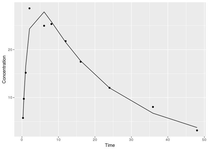
Great, we had successful convergence. Let’s see how the final fit looks.

preds <- pred(fit$par,observed=data,dosing=dose,mod=mod,param_names =names(params))[[1]]

print(ggplot(data,aes(x=V1,y=V2))+
        geom_point()+
        geom_line(aes(y=preds))+
        labs(x="Time", y= "Concentration"))

Generating standard errors of the parameter estimates

So far we know the parameter estimates to optimize our PK model, but we don’t know how precise they’re estimated. We’ll use finite difference approximation to approximate the Hessian matrix, and the negative inverse will provide the covariance matrix. Details on the functions used below are beyond the scope of this post. You can refer to the ADAPT5 user guide for more information on the calculation of the covariance matrix.

h <- function (atol,rtol,params){
  (rtol)^(1/2)*max(params,atol)
}
hj <- Vectorize(h,c("params"))

dydtheta <- function (params,hja,observed,dosing,mod,param_names){
  obs<-as.vector(unlist(observed[-1]))

  dydtheta.all <- matrix(0, nrow =length(obs),ncol=length(params))

  for (i in 1:length(params)){
    new_params <-params
    new_params1 <- new_params
    new_params2 <- new_params
    
    
    new_params1[i] <- new_params[i]+hja[i]
    new_params2[i] <- new_params[i]-hja[i]

    a1 <- pred(new_params1,observed,dosing,mod,param_names)
    a2 <- pred(new_params2,observed,dosing,mod,param_names)
    
    dydthetai <- (a1[[1]]-a2[[1]])/(2*hja[i])
    dydtheta.all[,i] <- as.matrix(dydthetai)
  }
  dydtheta.all
}

dgdtheta <- function (params,hja,observed,dosing,mod,param_names){
  obs<-as.vector(unlist(observed[-1]))

  dgdtheta.all <- matrix(0, nrow =length(obs),ncol=length(params))

  for (i in 1:length(params)){
    new_params <-params
    new_params1 <- new_params
    new_params2 <- new_params
    
    
    new_params1[i] <- new_params[i]+hja[i]
    new_params2[i] <- new_params[i]-hja[i]
    
    a1 <- pred(new_params1,observed,dosing,mod,param_names)
    a2 <- pred(new_params2,observed,dosing,mod,param_names)
    
    
    dgdthetai <- (a1[[2]]-a2[[2]])/(2*hja[i])
    dgdtheta.all[,i] <- as.matrix(dgdthetai)
  }
  dgdtheta.all
}

cov.matrix <- function(params,observed,dosing,mod,param_names){
  hja <- hj (mod@atol,mod@rtol,params)
  obs<-as.vector(unlist(observed[-1]))

  dydtheta.all <- dydtheta(params,hja,observed,dosing,mod,param_names)
  
  dgdtheta.all<-dgdtheta(params,hja,observed,dosing,mod,param_names)
  
  M <- matrix (0,nrow =length(theta),ncol=length(theta))
  variancepred<- pred(params,observed,dosing,mod,param_names)[[2]]


  M <- 1/2*(t(dgdtheta.all/(c(variancepred^2)))%*%(dgdtheta.all))
  M[1:length(theta),1:length(theta)] <- (M[1:length(theta),1:length(theta)]+ 
                                         t(dydtheta.all[,1:length(theta)]/c(variancepred^1))%*% 
                                          (dydtheta.all[,1:length(theta)]))
  
  
  
  cov <- solve(M)
  cov
}

cov<-cov.matrix(fit$par,observed=data,dosing=dose,mod=mod,param_names =names(params))

# Covariance matrix
print(cov)

.              [,1]        [,2]          [,3]          [,4]
. [1,] 0.0023631869 0.035726470  7.992320e-04  1.275675e-04
. [2,] 0.0357264704 2.875024690  7.927207e-02  2.623766e-03
. [3,] 0.0007992320 0.079272073  3.912149e-03 -4.236653e-10
. [4,] 0.0001275675 0.002623766 -4.236653e-10  4.723104e-04

# Calculate percent relative standard error 
RSE <- diag(sqrt(cov))/fit$par*100
names(RSE)<-paste("%RSE",names(params))

print(RSE)

.     %RSE CL     %RSE VC     %RSE KA %RSE sigma1 
.    3.560095    6.037265    9.959311   21.536089

# Correlation matrix
print(cov2cor(cov))

.           [,1]       [,2]          [,3]          [,4]
. [1,] 1.0000000 0.43343132  2.628549e-01  1.207473e-01
. [2,] 0.4334313 1.00000000  7.474665e-01  7.120174e-02
. [3,] 0.2628549 0.74746654  1.000000e+00 -3.116747e-07
. [4,] 0.1207473 0.07120174 -3.116747e-07  1.000000e+00

Fitting Pharmacokinetic/Pharmacodynamic Models Using R

A Brief Tutorial